Department of Biomedical Engineering
 
middle  
   
   
ANC Homepage
Block AP - Preliminaries
Unidirectional Propagation
Selective Activation
Electrochemistry
Tissue Response:
Brain |Nerve| Muscle
 
 
Links & Resources
Contact
 
BME Homepage


Previous - 1 - 2 - 3 - 4 - 5 - 6 - 7 - 8 - Next
 
Selective Activation: Part 1: Page 2

Selective Activation of Peripheral Nerves


Electrodes applied to most peripheral nerves can electrically access a large number of axons within the nerve. In many cases, advantage may be taken of the fascicular arrangement of the axons within the nerve trunk. By placing multiple electrode contacts around or within the nerve, the field of influence of the applied electrical stimulus can be directed to selectively activate subsets of axons within the nerve. In the figure, a radial arrangement of four electrical contacts is shown arrayed around a nerve trunk with four fascicles. By orchestrating the electrical field spatially and temporally from specific contacts, different subpopulations of the axons may be selectively activated.


Numerical Analysis of Electric Field Generated by a Nerve Cuff Electrode.

A 3-D finite element model of an unifascicular nerve was developed to study the potential distribution from a nerve cuff electrode [1]. A schematic model nerve is shown in the figure. The z-axis runs in the direction of the axons in the nerve trunk. The 3-D domain representing the nerve, surrounding tissue and the electrode were assumed purely resistive. The nerve model consisted of 28 layers with 256 volume elements along the axis of the nerve. A finer mesh was used in the region inside and close to the electrode.
The x-y and the x-z planes were considered to be two planes of symmetry. Therefore, only one-fourth of the problem was modeled using 7769 nodes and 1680 volume elements.
The electrical potential distribution was obtained by solving the Laplace Equation within a 3-D domain. The solution was obtained by minimizing a functional given by the equation at the bottom of the Figure.

Geometry of the Nerve

The geometry of the represented nerve is shown in the figure. It was modeled as a three-mm. diameter, unifascicular anisotropic structure with
s-longitudinal = 1.0 S/m and s-transverse = 0.1 S/m, surrounded by a 30 µm perineurium with sigma = 0.00063 S/m.
Two layers of encapsulation tissue, a 150 µm loose layer with s = 1.0 S/m and a 50 µm tight layer with s = 0.0659 S/m (so that the effective sigma = 0.22/m) and a 50 µm layer of 0.9% saline (sigma =2.0 S/m) were considered to between the nerve and the electrode.
The electrode contacts were 30 µm thick with s = 10^4 S/m and with surface area of 1.57 sq. mm. They were embedded on the inner surface of a 1 mm thick insulated nerve cuff (sigma = 10^-6 S/m). The surrounding body fluid was represented by a 20 mm layer of saline.


Previous - 1 - 2 - 3 - 4 - 5 - 6 - 7 - 8 - Next


. .  
Legal Information | 2004 - 2014 Case Western Reserve University | Contact
Updated : August 20, 2014
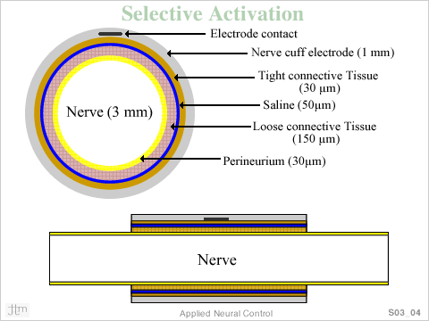